L. David Roper
http://www.roperld.com/personal/roperldavid.htm
May 2008
Slide Show for this web page
Mathematics of Global Warming
Global Warming web pages by L. David Roper
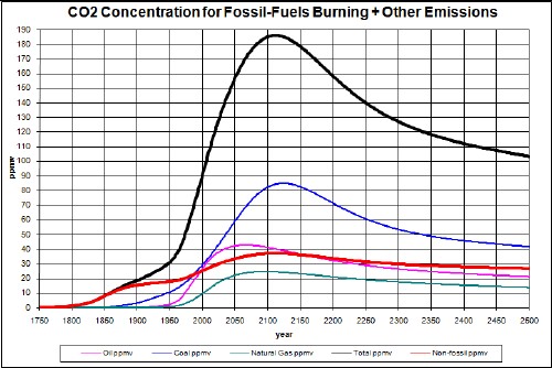
An approximate calculation is done of the carbon-dioxide concentration in the earth's atmosphere due to burning fossil fuels: coal, crude oil and natural gas. Since these are finite resources and the peak date for crude-oil extraction is about now, the peak date for natural-gas extraction will be about a decade from now and the peak date for coal extraction will be about year 2060, then carbon-dioxide atmospheric concentration due to burning fossil fuels will peak about year 2110, delayed about 100 years from the combined fossil-fuels emission peak because of the carbon-dioxide residence-time decay in the atmosphere.
Therefore, carbon emissions due to burning fossil fuels cannot increase indefinitely, which is some good news for future global warming. However, the impending decline of fossil-fuels extraction is not good news for societal stability and some unknown slow or future-triggered positive-feedback mechanisms may increase global warming more than the fossil-fuels emissions, non-fossil-fuels emissions and known fast positive-feedback effects.
An implicit assumption in this calculation is that humans will burn up or make chemicals from fossil fuels as fast as they can extract them from the earth. No account is taken in this work of global dimming (also see http://www.roperld.com/science/GlobalWarming_Dimming.htm) by atmospheric aerosols, which reduces global average temperature.
Adding an approximate calculation of deforestation and other non-fossil-fuels emissions to the fossil-fuels carbon emissions, assuming that non-fossil-fuels emissions are proportional to change in world population, yields a contribution to CO2 concentration that peaks at about 2025 with somewhat less magnitude than the contribution due to crude-oil burning. The combination of fossil-fuels burning and non-fossil-fuels emissions causes a CO2 concentration peak of about 450 ppmv at about year 2110, which corresponds to a temperature rise above year 2005 of about 0.5°C. The calculated concentration corresponds closely to measured values in past concentration-rising years from 1958-2007. And the calculated temperature rise of about 0.8°C from the 19th century to 2005 is close to the measured value.
A "wild card" is the existence of methane clathrates under the ocean and methane clathrates and carbon in Arctic permafrost that can react with oxygen to produce carbon dioxide, which may be released into the atmosphere as the permafrost melts before the fossil-fuels peak. Or humans may learn how to extract methane from clathrates and burn it for energy. Such releases of methane into the atmosphere or carbon-dioxide emissions from burning methane could greatly add to global warming. Fast positive mechanisms, such as reduced sunlight reflection due to melting ice and increased ocean surface, are presumably included in the climate sensitivity used to calculate temperature rises in this work, but there surely are some uncertainties. So the calculation reported here yields an approximate minimum for global warming due to fossil-fuels burning and non-fossil-fuels emissions. Appendix 3 gives a worst-case approximate calculation of temperature rise due to carbon release from permafrost melting. The result is a CO2 concentration peak of about 535 ppmv at about year 2125, which corresponds to a temperature rise above year 2005 of about 1.2 °C.
Another wild card is the possible sliding of the Greenland ice sheet into the ocean, lubricated by melt water that is draining underneath it. Similarly, the West Antarctica ice sheet may continue to break off at a faster rate. The disasters will be due to fast rising sea levels rather than increased temperatures.
There may be a competition between peak oil and global warming as to which one causes the greatest destabilization of world civilization. It appears that peak oil destabilization might occur first and then plentiful oil will not be available to ameliorate the disastrous effects of global warming.
The author has performed fits to fossil-fuels extraction data. Those fits are viewable at:
(Note that I use the word "extraction", not "production". Earth resources are "extracted", not "produced".)
The amount of eventual total extraction for coal, crude oil and natural gas predicted by the fits exceeds known resources; so they are optimistic predictions for future extraction. Curves for the fits are given in Appendix 1. To allow for possible large errors in known fossil-fuels resources, fits are also shown and used in the calculations for doubled eventual total extraction of the three fossil fuels.
These fits for fossil fuels are used to calculate the amount of carbon emitted into the atmosphere in future years by burning them. Then the increase in concentration of carbon dioxide in the atmosphere that those emission create is calculated. Finally, an approximate calculation of earth's average temperature change from the year 1700 value due to fossil-fuels burning is done.
Of course, there are other net emitters of carbon into the earth's atmosphere; such as deforestation, cement production, soil depletion and volcanic eruptions. Carbon-dioxide atmospheric concentration due to non-fossil-fuels emissions is added to the calculation by assuming that it is proportional to the change in population from the year 1700 into the past and into the future; its value for 2005 is known approximately for deforestation (about 1.6 gigatonnes/year), perhaps the largest contributor to non-fossil-fuels emissions.
Some factors are needed to do the calculations:
1 ton (2000 lbs) = 0.907 tonnes (1000 kg).
Carbon emitted = 12/44 CO2 emitted = 0.273 CO2 emitted.
Coal contains about 50% carbon by mass.
Crude oil contains about 84% carbon by mass [about average of C5H12 and C18H38 or (5/6 + 18/21)/2]
1 barrel of crude oil = 0.136 tonnes.
Natural gas contains about 76% carbon by mass [about 80% CH4 + 20% C2H6 or 0.8*3/4 + 0.2*4/5]
1 tcf (thousand cubic feet) of natural gas = 0.0189 tonnes.
CO2 concentration increment in ppmv = about 0.47 x gigatonnes carbon emitted.
Climate
sensitivity = 3 °C for doubling of CO2 concentration in the atmosphere.
2005 total carbon emissions = about 8 gigatonnes; about 20% is due to deforestation (about 1.6 gigatonnes)
An assumption is made that 25% of all three of the fossil fuels extracted are not burned; instead they are used to make useful compounds. This assumption could be relaxed to allow the burned-ratio to be different for the three different fossil fuels. Of course, it probably varies differently with time for all three of the fossil fuels. This factor of 25% could also include the inefficiency of burning the fossil fuel; that is, it could be the product of the fraction not burned intentionally and the fraction not burned due to inefficiency.
Actually, there are three numbers that multiply in calculating the carbon emissions for each of the three fossil fuels, the fraction of carbon in the fuel and the fraction of the fuel that is burned. They are:
Fossil Fuel |
Factor=FractionCarbon*FractionBurned |
coal (short tons to tonnes) |
0.907*0.5*0.75=0.375 |
crude oil (barrels to tonnes) |
0.136*0.84*0.75=0.63 |
natural gas (tcf to tonnes) |
0.0189*0.76*0.75=0.57 |
So, any combination of the two factors that yields the total could apply.
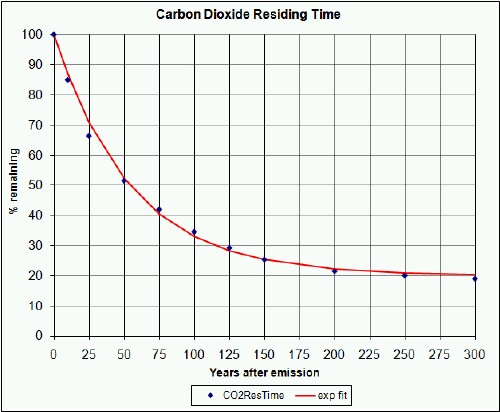
Carbon dioxide in the atmosphere has complicated interactions with the earth. Its removal from the atmosphere is not a simple exponential decay; about 10% is still in the atmosphere 1000 to 10,000 years after its emission. However, I have found that the removal data can be fitted reasonably well for the first 300 years after emission with an exponential having a 55-year time constant to a final 20%, which is a sufficiently long time for the calculations reported in this article:
That is, each year of emissions for any component (e.g., coal) is subject to this decay law. This is a little tricky to implement in MS Excel. For example, for each year after the first year of a CO2 concentration (in ppmv) calculation (=0.47*0.84*B1 for crude oil that contains about 84% carbon), the following formula is used to calculate the CO2 concentration in ppmv for crude oil for later years due to each year's emissions:
{=0.47*0.84*(B2+SUM($B$1:B1*(0.2+0.8*EXP(-(A2-$A$1:A1)/55))))},
where the brackets { }indicate an array calculation (SHIFT-CTRL-ENTER keys pressed after typing the entry).
In normal mathematical notation, the equation for the CO2 concentration (in ppmv) left in the nth year for the emissions in all the previous years is
 .
.
This array calculation applies the decay law to each year's emissions to get the amount remaining in the atmosphere in later years due to that specific year's emissions.
I also fitted the CO2 residence time with a decay curve that uses three decay times; there is very little difference for the next 300 years between the single-exponential and the three-exponentials fits. The three-exponentials decay law is used in all the calculations of this study to allow for a better extrapolation out to thousands of years.
Here is a graph showing the decay out to 10,000 years:
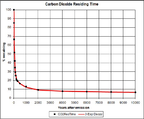
It goes to zero at infinity. Note that 20% is still in the atmosphere at 250 years, 10% is still there at 2000 years and 6% is still there at 10,000 years after emission.
The equation for the fit is
This array calculation applies the decay law to each year's emissions to get the amount remaining in the atmosphere in later years due to that specific year's emissions.
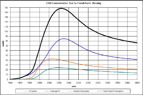
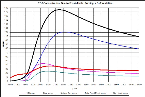
The factors needed to calculate the atmospheric CO2 concentration in ppmv due to coal emissions are given above and the extraction data and projection into the future are given in Appendix 1. After converting to gigatonnes/year and multiplying by 0.5 to get the approximate carbon content and by 0.47 to convert from gigatonnes of carbon emissions to ppmv CO2 concentration, the curve is obtained as shown in the graphs below.
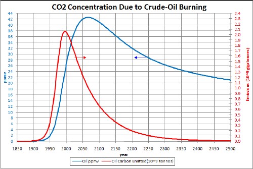
The factors needed to calculate the atmospheric CO2 concentration in ppmv due to crude-oil emissions are given above and the extraction data and projection into the future are given in Appendix 1. After converting to gigatonnes/year and multiplying by 0.84 to get the carbon content and by 0.47 to convert from gigatonnes carbon emissions to ppmv CO2 concentration, the curve is obtained as shown in the graphs below.
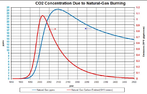
The factors needed to calculate the atmospheric CO2 concentration in ppmv due to natural-gas emissions are given above and the extraction data and projection into the future are given in Appendix 1. After converting to gigatonnes/year and multiplying by 0.76 to get the carbon content and by 0.47 to convert from gigatonnes carbon emissions to ppmv CO2 concentration, the curve is obtained as shown in the graphs below.
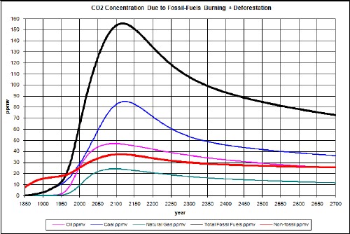
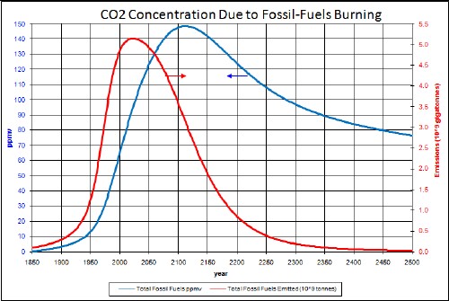
The calculated carbon emissions due to burning fossil fuels are in the following graph.
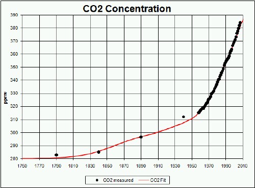
From the beginning of the current interglacial, about 10,000 years ago, until the discovery of coal and oil in the earth and the resulting population explosion, the CO2 concentration was approximately constant at about 280 ppmv from about 4000 years ago until large quantities of fossil fuels were discovered c1700. This gives a value to add to the fossil-fuels emissions concentration values calculated in this work.
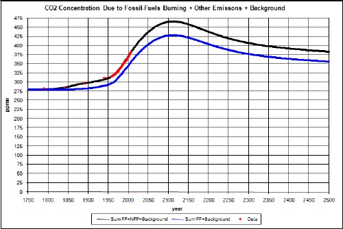
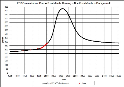
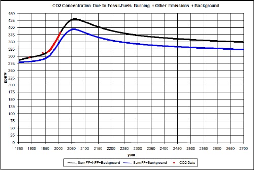
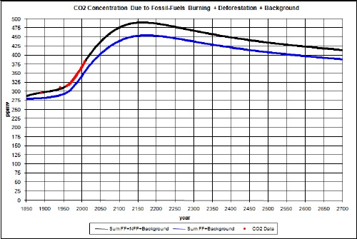
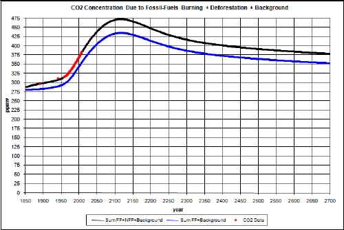
Now combine the total fossil-fuels atmospheric CO2 concentration with the background 280 ppmv:
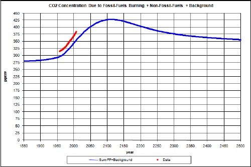
The red data points are the measured atmospheric CO2 concentration values at Mauno Loa Observatory, Hawaii. The fossil-fuels contribution to CO2 concentration are not enough to match the data, as expected. There are non-fossil-fuels emissions which must be approximated. It is interesting that the average slope of the data, measured for years 1958 to 2007, is about the same as the average slope of the fossil-fuels calculation.
See Appendix 2 for graphs that compare the carbon emissions to the atmospheric CO2 concentration for the three fossil fuels.
Besides fossil fuels carbon emissions, probably the next greatest source of carbon emissions is deforestation. The World Bank estimates that deforestation accounts for 20% of carbon emissions. The total carbon emissions for year 2005 were about 8 gigatonnes. So 20% is about 1.6 gigatonnes for deforestation emissions in 2005..
An approach to approximating the CO2 concentration contribution due to sources other than fossil fuels is to do a linear fit of the calculated fossil-fuels concentration (plus background) to the measured concentration data from 1958 to 2007 and Vostok-ice-core data since 1700. Rational for this approach is that the amount of deforestation, soil depletion, etc. is probably proportional to the amount of fossil fuels burned. Such a linear fit [![]() ] yielded a good fit except that the constant is too high; it should be about 280 ppmv instead of 292 ppmv. To get the pre-fossil-fuel rise from c1700 to c1900 a hyperbolic tangent in time was used, so that the fit equation is:
] yielded a good fit except that the constant is too high; it should be about 280 ppmv instead of 292 ppmv. To get the pre-fossil-fuel rise from c1700 to c1900 a hyperbolic tangent in time was used, so that the fit equation is:
![]()
The gentle rise from 280 ppmv to 295 ppmv before fossil fuels made large contributions is probably attributable to pre-fossil-fuels industrialization. Note that the non-fossil-fuels (NFF) contribution is about 14% of the fossil-fuels (FF) contribution, which is somewhat lower than it should be, according to some estimates. However, under the assumption that NFF is proportional to FF, the factor of the amount of FF extracted that is burned, the factor that converts carbon emitted to CO2 concentration and the fraction NFF/FF are multiplicative, so they can be varied in the opposite direction without affecting the results. For example, if the NFF/FF factor is changed from 0.14 to 0.5, the concentration factor is changed from 0.47 to 0.357. For an NFF/FF change of 0.14 to 0.25, the concentration factor change is 0.47 to 0.429.
Then the non-fossil-fuels CO2 concentration was calculated by subtracting the fossil-fuels CO2 concentration from the total CO2 concentration:
and
Note that the ~470 ppmv peak is very close to 500 ppmv, which appears to be the historical concentration upper limit for a glacial Earth.
A good feature of this approach is that it presumably includes the effect of the feedback of temperature on atmospheric CO2 concentration as well as other carbon emissions besides fossil fuels.
To calculate the temperature relative to year 1700 from the CO2 concentration in the atmosphere one needs the climate sensitivity, the amount temperature changes for a doubling of CO2 concentration. This number is supposed to include the effects of fast positive-feedback and negative-feedback mechanism. Estimates for climate sensitivity range from 1.5°C to 10°C.
A good case has been made for a short-term climate sensitivity of about 3°C and a long-term climate sensitivity of about 6°C. The latter accounts for much slower positive-feedback mechanisms than the former. I use 3°C in this work, since the calculations only extend to a few hundred years from now. To calculate the temperatures given here for a different climate sensitivity S, multiply the temperature changes given in this work by S/3.
A probability graph for climate sensitivity is:
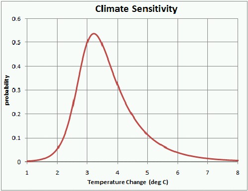
The curve is a Verhulst function with
Q |
1.039882 |
t1/2
|
3.473446 |
0.295616 |
|
n |
3.15563 |
Besides the climate sensitivity, one should allow for the fact that the ocean absorbs much of the solar energy impinging on the Earth and then slowly heats up the atmosphere. There is a climate response function that represents the atmospheric temperature time delay after carbon is inserted into the atmosphere. The function is
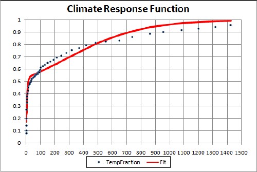
The two-hyperbolic-tangent fit is good because the data errors are large. The function is
![]()
A better fit could be obtained with three hyperbolic tangents, but the errors on the data do not justify it.
I use a climate sensitivity of 3 degrees celsius for CO2 concentration doubling to calculate the approximate temperature change relative to year 1700, dT (in Celsius degrees), due to a change in CO2 concentration, Ci (in ppmv). The equation is:
 or, equivalently,
  , where
 ![]() .
.
for year i from the concentration C0 for a reference year (1700 AD). The s factor is the climate sensitivity (assumed equal to 3 in the calculations done here) that makes the climate sensitivity factor be for doubling of the CO2 concentration in the atmosphere, as it is defined. (Climate sensitivity is supposed to include the effects of fast feedback mechanisms, both positive and negative, in other variables caused by changing the CO2 concentration.)
To account for the climate response time, the equation must be altered as follows:

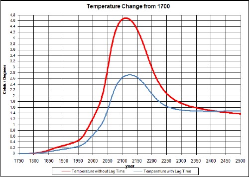
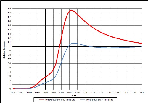
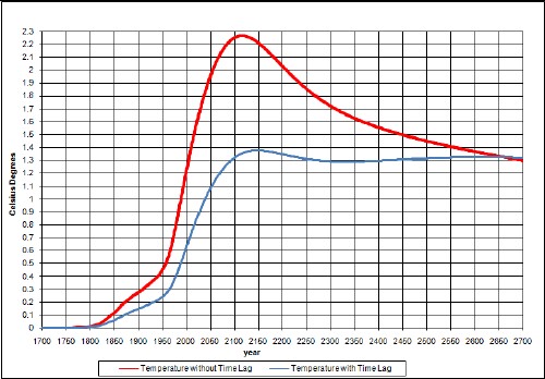
The resulting temperature change relative to 1700 due to fossil-fuels burning and non-fossil-fuels emissions is:
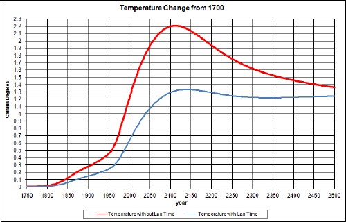
The upper curve is without taking account of climate response time and the lower curve takes it into account. The lower curve agrees well with measurements.
An unknown amount of global dimming should be subtracted from this curve; it is probably only a few tenths of a degree or smaller and quite variable with time.
The peak would be higher if it were not for the time delay between carbon emission and the atmospheric temperature. The asymptotic temperature is the same for both calculations, even though the ocean keeps some of the energy, because the climate sensitivity accounts for that.
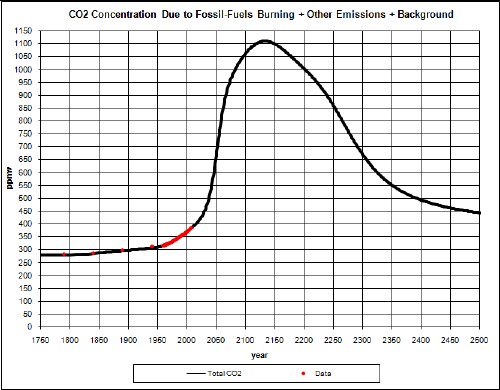
It may be that the amount of CO2 that can be taken out of the atmosphere by vegetation and the oceans is a decreasing function of the CO2 concentration. I did a calculation assuming that the 0.47 factor to multiply CO2 emissions to get CO2 concentration rises to twice that value according to
 .
.
The resulting CO2 concentrations and temperatures are:
The upper curve is without taking account of climate response time and the lower curve takes it into account.
So, if the amount of CO2 concentration in the atmosphere is increased by not being absorbed by vegetation and the oceans, the Earth average temperature could be considerably higher than the constant 0.47-factor case. The ~2.8°C temperature rise above the 1700 temperature given by this calculation would truly be disastrous for human civilization. (Six Degrees: Our Future on a Hotter Planet by Mark Lynas.)
The result of this calculation came as a very big surprise to me, because I had been assuming in my talks and web pages about global warming that the temperature would continue to rise to large values from the present temperature due to burning fossil fuels. Although I had done much work about fossil-fuels depletion, I had not applied that work to global warming until I did the work for this article.
So, this reasonable calculation indicates that global temperature will not rise to high values due to fossil-fuels burning, non-fossil-fuels emissions and, represented in the climate sensitivity, fast-feedback mechanisms. However, cheering should be muted because already disastrous results are occurring due to the approximate 1°C temperature rise from the 1900 to 2005; the predicted continuing rise up to 2100 of about 1°C above 2005 will accelerate those undesirable changes. And some surprises, such as massive releases of methane from permafrost thawing, could drastically change earth temperature in the future. ( Appendix 3 gives a worst-case approximate calculation of temperature rise due to carbon release from permafrost melting.)
There may be a competition between peak oil and global warming as to which one causes the greatest destabilization of world civilization. It appears that peak oil destabilization might occur first and then plentiful oil will not be available to ameliorate the disastrous effects of global warming.
Suppose that we learn how to sequester some of the carbon from coal before or after we burn it or we institute a gradual moratorium on burning coal. For purposes of doing an approximate calculation, assume that the amount of carbon put into the atmosphere by burning coal is modified as a function of time by the factor shown here:
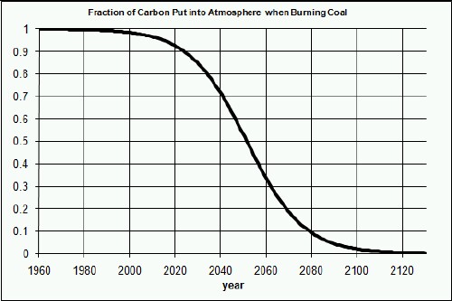
which is a plot of the function ![]() . This corresponds to about a hundred-year time interval to achieve full carbon sequestration or to completely stop burning coal.
. This corresponds to about a hundred-year time interval to achieve full carbon sequestration or to completely stop burning coal.
The results of the calculation are:
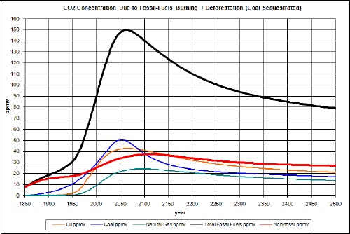
The coal peak is slightly higher than and at about the same time as the crude-oil peak The coal peak occurs at about 2050 instead of 2125.
The peak is about 425 ppmv but then the ppmv reduces to an asymptote at about 360 ppmv. Compare to about a 380 ppmv asymptote without coal carbon sequestration or a coal moratorium. That is, it is already too late to begin to greatly reduce the peak or the asymptote by very much by carbon sequestration or a moratorium on burning coal.
The upper curve is without taking account of climate response time and the lower curve takes it into account.
The temperature-change peak is about 1.1°C relative to the year 1700 temperature. So, the temperature peak is reduced about 0.3°C by this amount of carbon sequestration.
Suppose by some miracle that twice as much coal (3 x 10¹² tons) is able to be extracted from the earth than assumed in the fit to coal-extraction data used above (1.5 x 10¹² tons). The results are:
The upper curve is without taking account of climate response time and the lower curve takes it into account.
The temperature-change since year 1700 does not peak; it just climbs for hundreds of years.
Suppose by some miracle that twice as much crude oil (4 x 10¹² barrels) is able to be extracted from the earth than assumed in the fit to crude-oil-extraction data used above (2 x 10¹² barrels). The results are:


The upper curve is without taking account of climate response time and the lower curve takes it into account.
The temperature-change peak is about 1.4°C above the year 1700 temperature, only about 0.1°C more than for the case for half that eventual crude-oil extraction.
Suppose by some miracle that twice as much natural gas (30 x 1012 tcf) is able to be extracted from the earth than assumed in the fit to natural-gas-extraction data used above (15 x 1022 tcf). The results are:

The upper curve is without taking account of climate response time and the lower curve takes it into account.
The temperature-change peak is about 1.4°C above the year 1700 temperature, about 0.05° higher than the case for half that eventual natural-gas extraction.
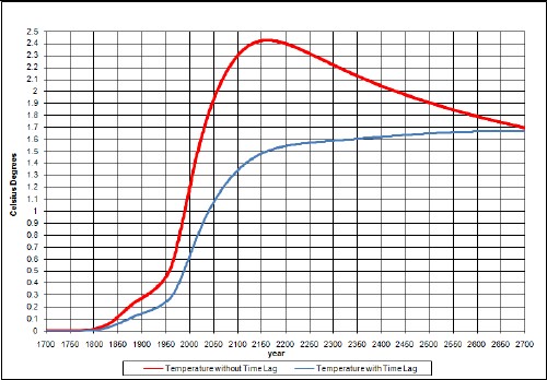
Putting together the most likely fossil-fuels depletion, the CO2 feedback and the possibility of carbon release by Arctic tundra melting, the following results are obtained:
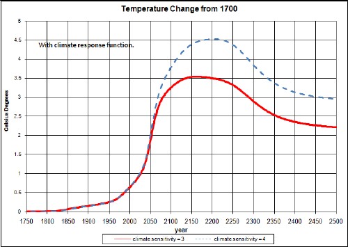
The dashed curve is for a gradual climate sensitivity change from 3 to 4.
So, we see that there would be terrible catastrophes for human life. (See Six Degrees: Our Future on a Hotter Planet by Mark Lynas.)
If no other large sources of carbon emissions exist or occur in the future, the peaking of crude oil, natural gas, coal and deforestation/non-fossil-fuels emissions (due to the peaking of population growth) will keep carbon emissions from rising to extremely high values, barring massive releases of methane from the ocean and arctic permafrost (see Appendix 3) or other unknown slow or future-triggered positive-feedback mechanisms. The resulting peak of CO2 concentration will occur at about 2100 at about 450 ppmv with a leveling off at about 380 ppmv for the next several hundred years or so.
The temperatures calculated for all the cases considered in this work, including the appendices, are:
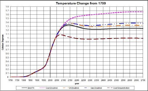
The top dotted curve is for coal doubled and the bottom dashed curve is for carbon sequestration or a moratorium on coal burning. I doubt that carbon sequestration/moratorium will occur nearly as much as calculated here, and coal doubling is extremely unlikely.
The weak part of this calculation is probably the calculation of non-fossil-fuels emissions of carbon into the atmosphere. The author would welcome suggestions about how to do that better.
A "wild card" is the existence of methane clathrates under the ocean and methane clathrates and carbon in Arctic permafrost that can react with oxygen to produce carbon dioxide, which may be released into the atmosphere as the permafrost melts before the fossil-fuels peak. If humans learn how to extract methane from methane clathrates for fuel, perhaps much more carbon will be put into the atmosphere. (Methane decays with a half life of about 7 years into carbon dioxide.) Increased earth temperatures may cause some of the methane clathrates to release methane into the atmosphere. Already methane clathrates in Arctic permafrosted tundra are releasing methane at a rather high rate due to rising temperature. There is a huge amount of carbon trapped in the permafrost of tundra, which would oxidize into carbon dioxide if the tundra thaws. Appendix 3 gives a worst-case approximate calculation of temperature rise due to carbon release from permafrosted tundra melting.
I believe that humans will continue to extract and burn fossil-fuels as fast as possible. Fortunately, the peaking of fossil-fuels extraction will put a natural brake on that burning. Unfortunately, the peaking of fossil-fuels extraction will cause massive disruptions in meeting the sustenance needs of nearly 7 billion humans. Also, the increase in temperature in about the year 2100 of about 1.4°C (2.5°F) above the 19th-century temperature will cause great suffering. The current emphasis on cutting back carbon emissions from fossil-fuels burning is needed to reduce global warming, but even more to preserve the fossil fuels for making useful materials and to prepare society for the economic disruptions that will undoubtedly occur when the populace finally realizes that we are on the down side of fossil-fuels depletion.
Probably the best that we can corporately do is to plan for the disruptions that will occur, both from the increase in temperature until 2100, and possibly on into the future if methane clathrates come into play, and the decline of availability of fossil fuels. However, we should strenuously try to use fossil carbon compounds for useful materials instead of burning it for energy.
I have also done a calculation of energy supplied by fossil-fuels burning.
After this work was completed I found the following similar analyses of fossil-fuels burning and global warming:
A summary of the mathematics used in this work.
The asymmetric peaked Verhulst function is used to fit the fossil-fuels extraction data:
 ,
,
where 
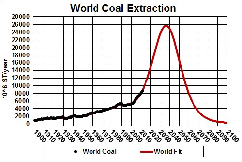
The total amount to be extracted (area under the curve) is 1.5 x 10¹² tons for the blue curve and 3 x 10¹² tons for the red curve.
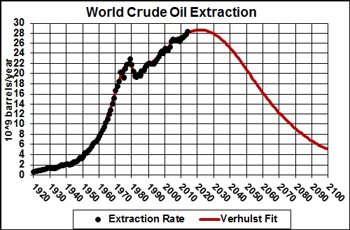
The total amount to be extracted (area under the curve) is 2 x 10¹² barrels.
The following curve contains information that probably will have the greatest effect on those now living and born in the future:
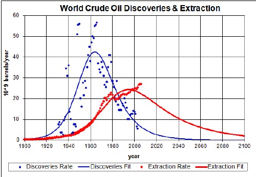
The amount under both curves is about 2x10¹² barrels.
Crude Oil cannot be extracted if it has not been discovered! So far the amount extracted has exceeded 1x10¹² barrels, so we are more than halfway there!
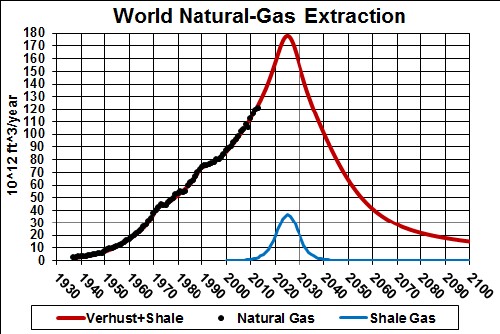
The total amount to be extracted (area under the curve) is 15 x 1015 ft 3 = 15 x 1012 tcf.
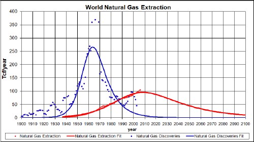
The amount under both curves is about 15 x 1012 tcf.
Natural gas cannot be extracted if it has not been discovered!
 t
t
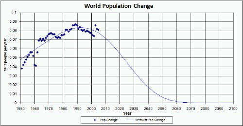
The bottom graph shows the change in population, with a peak at about 1990-95.
The following graphs compare the carbon emissions to the carbon-dioxide concentration in the atmosphere for fossil-fuels burning and non-fossil-fuels emissions:
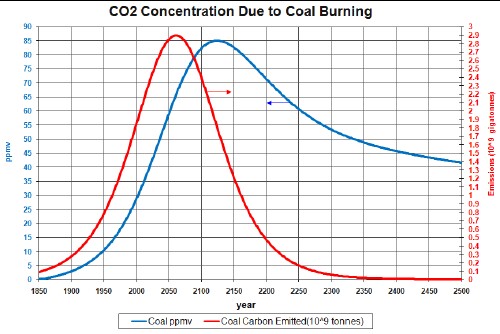
Coal emissions and ppmv
Crude-Oil emissions and ppmv
Natural-gas emissions and ppmv
All fossil-fuels (coal, crude oil and natural gas) emissions and ppmv
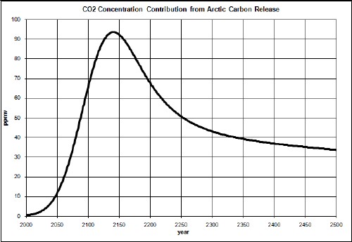
The amount of carbon stored in the Arctic permafrost is estimated at 500-2500 gigatonnes. As an example case, assume 400 gigatonnes of carbon is released according to the following Gaussian function:
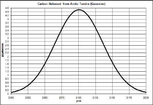
That is, it is a release over a time interval of about 100 years with a width of about 50 years. The area under the curve is 400 gigatonnes. (See http://thinkprogress.org/romm/2011/12/19/392242/carbon-time-bomb-in-arctic-new-york-times-print-edition-gets-the-story-right/ .)
The CO2 concentration caused by that release would be:
Adding this to the results obtained above, the total CO2 concentration would be:
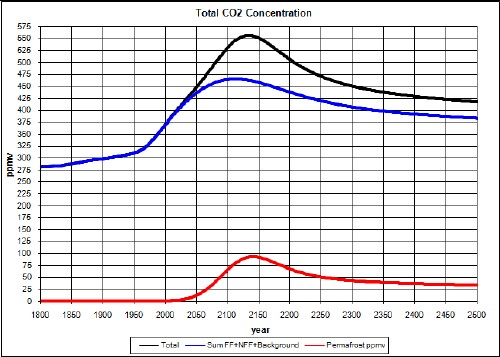
So, the CO2 concentration would get near to 550 ppmv.
The temperature change from year 1700 that this would cause is:
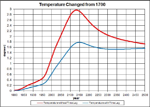
The temperature peak at about 2140 is about 1.7°C above the 2005 temperature.
The WEAP model makes cogent arguments that peaking of fossil-fuels extraction will cause a population reduction at about the middle of the 21st century by birth control or disasters or both.
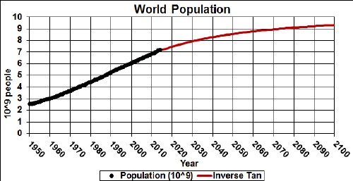
An approach for population decline or collapse is to assume that world population is proportional to the amount of fossil-fuel energy that is available. I did such a calculation which is shown in the following graph:
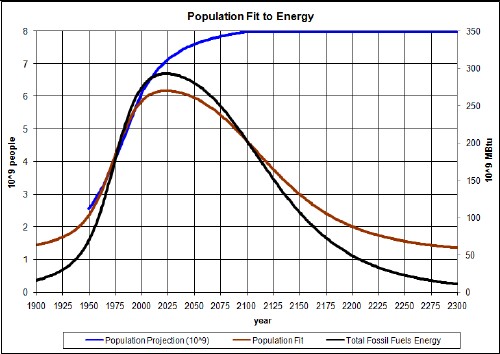
The blue curve is a population projection assuming approach to an asymptote of 8x10⁹ people. The brown curve is a population projection in which the population between 1950 and 2006 is fitted to the fossil-fuels energy available (unit 109 MBtu). The fit equation is
P = 1.350+0.01616*E.
It is seen that the population declines rapidly and approaches an asymptote of about 1.35x10⁹ people.
This more severe population reduction only reduces the peak and asymptotic temperatures by about 0.2°C.