L. David Roper
http://arts.bev.net/roperldavid
30 March, 2020
At first glance it may appear to be a mystery as to why so many of the events of the Universe can be modeled with mathematics. Some have declared that the Universe is just a super-giant computer which, of course, uses mathematics to do its calculations. (Arianrhod, 2003)
This article deals with a sub-mystery of the mathematics mystery in trying to explain why so many events of the Universe can be modeled to varying degrees of accuracy by the simple mathematics function, the hyperbolic tangent, whose definition (http://en.wikipedia.org/wiki/Hyperbolic_tangent) is
| (1.1) |
(e is the irrational number 2.71828183….
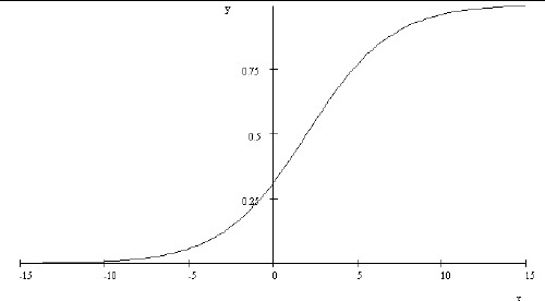
See http://en.wikipedia.org/wiki/Exponential_function.) The following is a graph of the hyperbolic tangent.
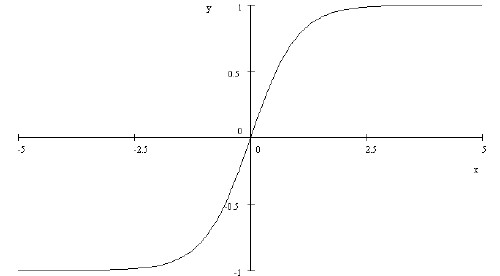
The popular press calls this the S-Curve.
The hyperbolic-tangent has interesting asymptotic properties:
 |
(1.2) |
Note that if x = y/t, where t is a time constant for the exponential behavior near x = 0, the hyperbolic time constant is twice the exponential time constant.
The following graph shows the hyperbolic tangent and the (e2x-1) function plotted together.
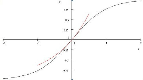
So we see that the following holds:
 |
(1.3) |
This function is shown in the following graph.
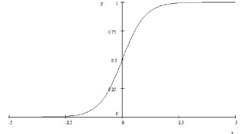
Note that the function of Eq. (1.3) has the very nice property of being zero for large negative x and 1 for large positive, having gone through 0.5 at x = zero. One can multiply this function by any number to model many natural phenomena which start at zero for some parameter #1 for a large negative value of parameter #2 and then exponentially rise near zero for parameter 2 and then asymptotically approach the multiplying constant for parameter #1 at large parameter #2.
Other useful combinations are:
The parameter t0 is the value of t where the slope changes from increasing to decreasing, the "break" or "inflection" point.
A more general function is needed for real-World fits to natural phenomena, as given in the following equation.
 |
(1.4) |
For example,  is shown in the following graph.
We see why the parameter symbols w and p were chosen in the more general hyperbolic tangent in Eq. (1.3) when we take the derivative of the function.
 |
(1.5) |
For example,  is shown in the following graph.
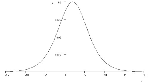
We see that the equation’s parameters have the following meanings:
Sometimes natural data are in the form of an asymptotic curve such as Eq. (1.4) and sometimes natural data are in the form of a peaked curve, such as Eq. (1.5). As shown above, they are related by a calculus derivative, or inversely a calculus integral.
For minerals depletion (Roper, 1976) the relevant equations are
 |
(1.7) |
It is rare that natural peaked data are symmetrical about the peak; similarly asymptotic data often have a different rate going into the asymptote than the growth rate from zero. One needs a generalization of the hyperbolic tangent that allows such asymmetry. Such a generalization, the Verhulst function, is derived in (Roper, 1976).
 |
(1.8) |
For n = 1 Eq.(1.8) reduces to Eq. (1.7), the symmetric case. For 0 >= n >= 1 skewing is toward short times and for n < 1 skewing is toward large times.
Now that we have seen the mathematical shape of the hyperbolic tangent it is not so mysterious why it is applicable to so many physical processes. Many physical processes have several different states of existence. The hyperbolic tangent is a function that can easily represent the transition from one state to another. The general form for a double hyperbolic tangent is:
Its value is a for large negative t, b for intermediate t and c for large postive t.
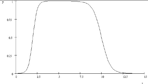
For turning on and then off a state the following function works quite well:
 |
(1.9) |
For example, the following graph shows the two transitions represented by ![]() .
.
Similarly, a useful triple-hyperbolic-tangent function is:
 .
.
Its value is a for large negative t, b for left-intermediate t, c for right-intermediate t and d for large postive t.
It is obvious how to generalize this equation for more than three (N-1) hyperbolic tangents:
This represents N hyperbolic tangents and N+1 levels, the first level with subscript 0 and the last with subscript N. A common case, e.g. for a virus epidimic, the initial level is 0. Then one can use a sum of terms given by Eq. 1-3 above with factors An.
Hyperbolic-tangent functions can be use to represent cumulative production of a product that changes between levels of daily/weekly/annual production. To do this the integral of the tanh function is needed to give the area under the production curve:
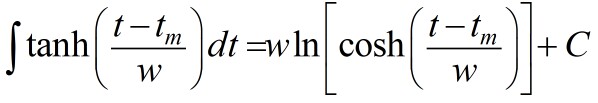
where C = integration constant which should be set to the value of the initial hyperbolic tangent in the series well before the transition to the first tanh, the value a in the equations given here.
For example, the double-tanh series for production
needs to have the value of C determined by this equation:
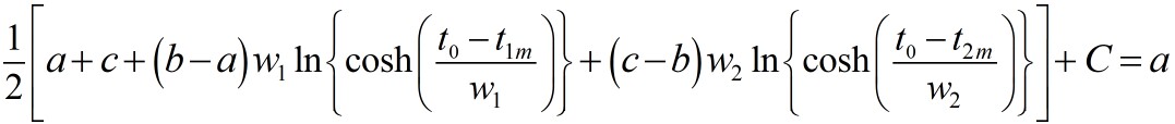
where t0 is a location well before the transition of the first tanh. This value of C is then inserted in the function
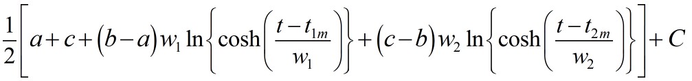
to calculate the cumulative production.
For an example of this see Production of Tesla Model 3 Electric Car.
It appears that World population growth is beginning to decline. The ideal situation would be that it would approach an asymptote rather than continuing to grow exponentially or disastrously decline by terrible calamities. A Verhulst function can be fitted to the data since 1950 to yield the curves shown in the following graph.
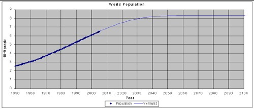
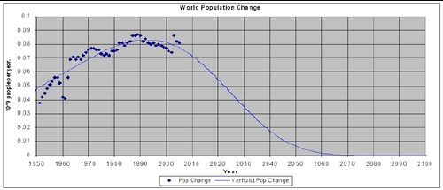
For a more detailed analysis of World population see (Roper, 1977).
The rate of crude oil extraction (“extraction”, not “production”!) in the United States is shown in the graph below.
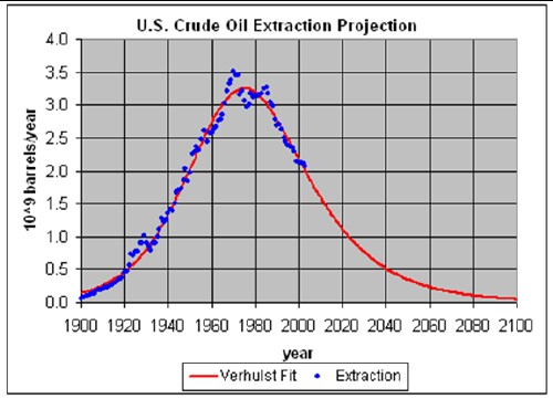
It peaked about 1970, got a slight boost from Alaska extraction in the 1980s, but has declined steadily for the last twenty years and will continue to do so with possible short-lived small peaks. The Verhulst function fit (Roper, 1976) to the data gives a reserves value 1.5 times the 2003 proven reserves, which probably is about right for predicting the future.
Note that the extraction curve is not symmetrical; it is skewed toward future times. This is to be expected as Herculean efforts will be made to extract crude oil in the future.
The graph below shows crude oil discoveries rate. Note the peak in discoveries at about 1965 and the rapid fall since about 1975. The Verhulst function fit (Roper, 1976) to the discoveries data gives the total amount of crude oil to be extracted as slightly less than 2 x 10 12 (2 trillion) barrels. Obviously, World crude oil discoveries have been meager and declining for the last thirty years.
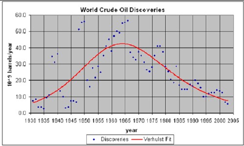
Extraction rates for crude oil are typically about forty years behind discoveries rates. So, the World crude oil extraction rate is expected to peak at about 2005.
The graph below shows the World crude oil extraction rate and two mathematical fits to the data. The two Verhulst-function fits (Roper , 1976) were obtained by fixing the total amount of World crude oil to be extracted at 2 x 10¹² (2 trillion) barrels, an amount consistent with the fit to World crude-oil discoveries discussed above and at 3 x 10¹² barrels, 50% more than the amount that fits the discoveries-rate data.
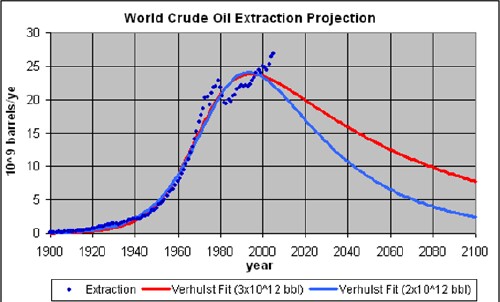
The peak has been predicted by many geologists to be between 2000 and 2010. (Deffeyes, 2005)
Whether the peak of crude oil extraction has already occurred or will occur in the near future, the message is the same: The World, led by the United States, must use the remaining crude oil mostly to develop the infrastructure needed for the use of renewable energy sources beginning now and into the future.
For more information about crude oil depletion see (Roper, 2005) and (Roper, 2006).
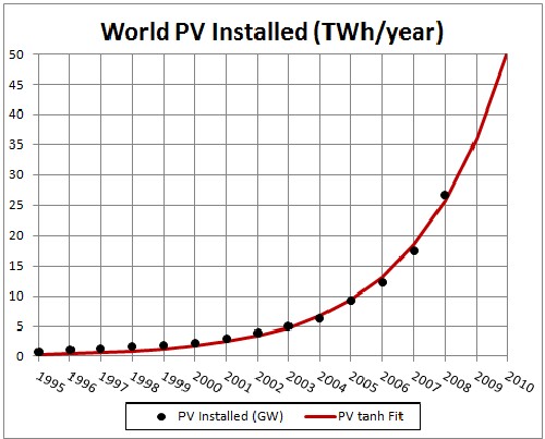
The eminent depletion of fossil fuels makes is necessary to develop renewable energy sources as soon as possible. A particular renewable energy starts off being used exponentially with time and finally levels off exponetially to an aysmptote; i.e., the the manner of the hyperbolic tangent.
Here is an example for solar photovoltaic energy:
The data points are cumulative PV installations. |
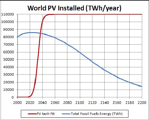
A comparison of the projected PV capability with fossil-fuels energy. |
Ice cores from Vostok Antarctica have yielded temperature data for the last 422,000 years. In that period of time there were four Major Ice Ages of about 115,000 years duration each.
In (Roper, 2004) it is shown that those last four Major Ice Ages can be reasonably fitted with Earth states transitions represented by hyperbolic tangents. The mathematical equation used to make the fits is
The fits to the last four Major Ice Ages and predictions for the next two Major Ice Ages are shown in the graph below.
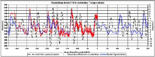
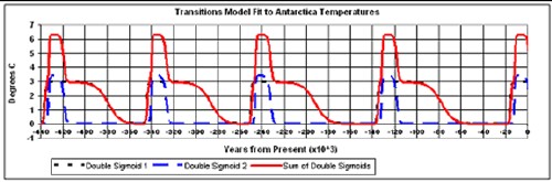
This is a fit to Antarctica temperature data for the last four Major Ice Ages by a mathematical function involving the North-Pole summer insolation and two Earth-states transitions in the time vicinity of the five Major Interglacials (Roper, 2004). The fit is then projected into the future for the next two Major Ice Ages. The bottom graph shows the two Earth-states transitions and their sum (solid curve).
For more details see (Roper, 2004).
Recycling is started being calculated at a specified initial year, t0, at a certain initial rate (Ri) and smoothly changes to a final recycling rate (Rf) according to the hyperbolic-tangent function: R = [Rf + Rf]/2+ [Rf - Rf]tanh[(t - tb)/w]/2 . The break point of the hyperbolic tangent is tb and the width is w.
Recycling of the mineral extracted in a specific year, ti, is not recycled until some later year. If fact, it is spread out over a range of years. That spread is assumed to be a Gaussian function centered at some later year, ti + tp with width wp. The total recyling function for year t after initial year t0 is:
This spreads out the extraction over a larger span of years. Thus, the mineral is spread out in time as well as in space as it is used to make items of use to humans.
The first recycling of a mineral will also be recycled a second time, which further spreads it out over time according to the recycling function, as well as further spreading it out over space.
The second recycing will be recycled a third time. This repetition continues until the spread in time is so large that it contributes a negligible amount to the useable material.
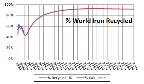
One has to make reasonable guesses about the values to use for the parameters for a given mineral. Here is a calculation for iron-ore extraction and recycling:
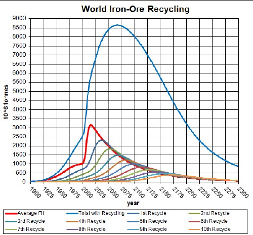

The parameters in the recycling equation above were determined by fitting the iron/steel recycling data for the United States, thereby assuming that the world recycling rate was similar:
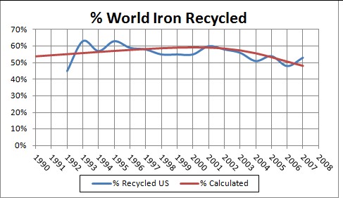
The recycling data are the ratio of recycled material to consumed material, rather than recycled material to extracted material. So, they are only an approximation to the real yearly recycling rate, since it does not account for imported material into the US. Also, the ratio of recycled material to extracted material is not what is referred to as "recycling rate" in the equation above; the equation rates are the ratio of recycled material to the extracted material in the same year in the past.
For more details see:
The time dependence of the “action potential” across the excitable membrane of the axon of a nerve cell can be represented by a combination of several hyperbolic tangents. (See http://en.wikipedia.org/wiki/Action_potential, http://en.wikipedia.org/wiki/Membrane_potential, http://en.wikipedia.org/wiki/Nernst_equation, http://en.wikipedia.org/wiki/Axon, and http://en.wikipedia.org/wiki/Hodgkin-huxley_model .)
A typical action potential (inside relative to outside) is shown in the graph below.
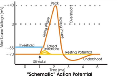
The explanation for the action potential, which once generated travels down the nerve axon with a speed of 10 to 100 meters/second, is as follows:
The opening of the two ion channels can be represented mathematically by two double hyperbolic tangents:
An example of a calculated action potential is shown in the following graph.
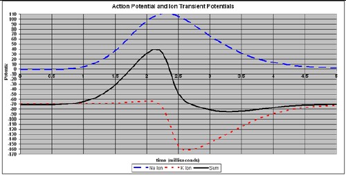
The parameters for this curve are:
V r = -70 |
C |
t1 |
w1 |
t2 |
w2 |
Na parameters: |
300 |
2 |
0.5 |
4 |
0.75 |
K parameters: |
100 |
3 |
0.1 |
4 |
0.4 |
These curves do not contain the transient stimulus electric potential of about +40 mV. It can be subtracted out from the measurement. It could be added to the equation as another double hyperbolic tangent.
If more ions are involved with channels opening, such as Ca ++, they can be added as another double hyperbolic tangent.
It would be interesting to try to obtain an approximation to the Hodgkin-Huxley equations (http://biolpc22.york.ac.uk/hh/hh_excel.html) for the action potential by mathematically manipulating the equation given here.
For details about fits to voltage-clamp data see http://www.roperld.com/science/NerveExcitation.pdf .
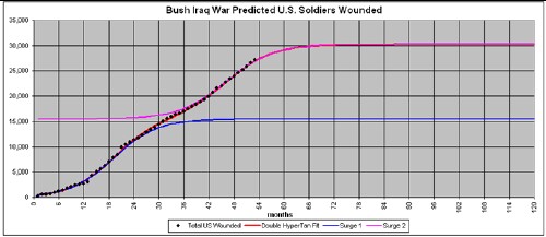
The Bush Iraq War had two “surges” of United States troops involved from its beginning in March 2003 to the end of 2007. Those two surges are very well fitted by two hyperbolic tangent functions as shown in the following graph:
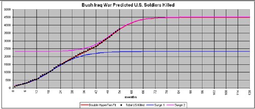
The parameters of the fit to the number killed are:
The parameters of the fit to the number wounded are:
Life expectancy at birth in the United States appears to have almost reached a plateau:
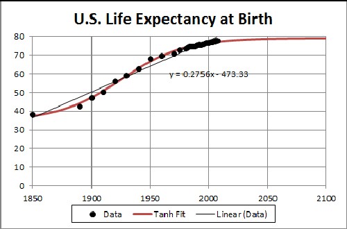
For more details see (Roper2010a).
The Standard and Poor's representation of the United States stock market can be represented as a sum of many states' changes using the hyperbolic tangent. Here is an 50-hyperbolic-tangent fit to date between the years 2000 and 2005:
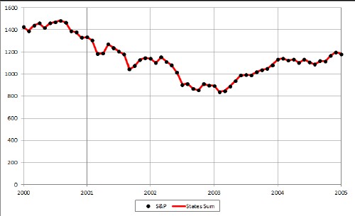
For more details see (Roper2011a).
A possible measure of human intelligence evolution is brain-to-body mass ratio, called the encephalization quotient (EQ). Here is an hyperbolic-tangent fit to the rough data:
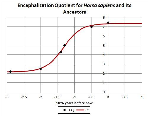
For more details see (Roper2010b).
Arianrhod, 2003: Einstein’s Heroes, Robyn Arianrhod, Univ. of Queensland Press, 2003.
Bartlett, 2004: The Essential Exponential: For the Future of Our Planet, Albert A. Bartlett, Univ. of Nebraska, 2004.
Roper, 1976: Depletion Theory, L. David Roper, http://www.roperld.com/science/minerals/DepletTh.pdf, 1976.
Roper, 1977:Projection of World Population, L. David Roper, http://arts.bev.net/roperldavid/WorldPop.htm, 1997.
Roper, 2004: Major Ice Ages Earth-States Transitions, L. David Roper, http://www.roperld.com/Science/TransitionsModelMIA.pdf, 2004.
Roper, 2005: World and United States Crude Oil Depletion, L. David Roper, http://www.roperld.com/science/minerals/FossilFuels.htm, 2005/2012.
Roper, 2006: Triple Threats for the Human Future: Will Civilization Arrive, L. David Roper, http://www.roperld.com/science/HumanFuture.pdf, 2006.
Roper, 2010a: Life Expectancy in the United States:
Roper, 2010b: Human Intelligence Evolution, http://www.roperld.com/science/humanintelligenceevolution.htm
Roper, 2011a: Stock Market as States' Changes, http://www.roperld.com/science/Stockmarketasstateschanges.htm
L. David Roper, http://arts.bev.net/roperldavid, roperld@vt.edu
See http://www.roperld.com/HumanFuture.htm