Projection of World Population
L. David Roper (roperld@vt.edu)
Blacksburg, Virginia 24060
ABSTRACT
A generalized version of the inverse tangent function is devised and found to yield an excellent fit to the World population data. All other functions that have been fitted to World population data yield c2 (goodness-of-fit parameter) values of three to four times greater than the c2 for the generalized inverse tangent function fit; i.e., the inverse tangent function is by far the best fit to the data. The parameters of the function are precisely determined by the data, one of them being a final World population of 6.0 billion. World population is projected to be about five billion in 2000 and 5.5 billion in 2050. This is in reasonable agreement with Lester Brown's timetable for World population stabilization. This work was done in 1978.
Introduction
Many attempts have been made to project the population of numerous geographical areas of the World and of the entire World. Probably the most
Putnam (1) and by Hart (2). Most projections use the logistic curve (3) or a sum of logistic curves to fit the past population data and thereby project the population into the future. We shall discuss below the more recent projections that utilize other functions. These projections of national populations have not been very accurate for various reasons:
· Large fluctuations often occur because of the small sizes of the populations.
· Immigration and emigration complicate the situations.
· The logistic function is restricted to exponential growth for early times and does not allow any asymmetry.
We shall show herein that an excellent fit to the World population data using a more general function than the logistic function is a good projector for the past decade; therefore, it is presented as the best available projector for the future.
Similar projections have been done for resource depletion, the best known of which is Hubbert's work on oil depletion (4) which utilized the logistic function. Lasky (5) used this method two decades ago for some metals. Recently (6) my colleague, Dr. Richard Arndt, and I have expanded this method of resource depletion projection by using several other functions besides the logistic function, including the Verhulst function (7), which is a generalization of the logistic function that allows for asymmetry in production. We found that, in many cases, some other function besides the logistic function fitted the data best. In fact, for most of the several U.S. metals that are past their production peaks the Verhulst function is required there is visible asymmetry even to the naked eye. For most of the World production data we found that the best fit was by means of the Lorentzian function (the derivative of the inverse tangent function), because the function has a longer tail than the logistic or Verhulst functions. We knew of no asymmetric generalization of the inverse tangent function and were not too concerned about devising one because very few world minerals have peaked in production. In subsequent work (8) we have shown that the asymmetry to occur later in United States mineral production data is often forecastable by fitting the Verhulst function to early data before the production peak. Perhaps the same would be true for World mineral production data if we had an asymmetric version of the inverse-tangent function to use in fitting the World data.
The relevance of the paragraph above to the projection of World population is twofold:
· The World population data show a long early time tail similar to the World mineral production data.
· One should allow for the possibility of asymmetry in fitting the data with functions to be used for projection.
A generalized version of the inverse tangent function that allows asymmetry is reported in this paper. This function yields a c2 (goodness of fit-parameter) for the fit (9) that is three to four times smaller than the c2 for the fits of any of the other functions that have been used to fit World population data. This means that our function yields a much more probable fit to the data than do the other functions. This best fit to the World data through 1975 yields a final population of 6.0 billion and a growth rate peak date of 1966. This is a surprisingly low projection for the World final population; it is more than four billion less than the United Nations projection.
Since the fit reported here is such an excellent fit to the data (indeed, by far the best fit of any function that has been used) and since its projection is excellent over the last decade, its projection into the future must be taken seriously.
World Population Data
Table 1 lists the World population data (41 data points) that are used in the fits, along with the references and estimates of errors that were obtained by means of the differences among different references for the same dates.
Table 1. World Population Data and References
Reference Date Population (10 9 Error (10 9 Reference Date Population
Error
Putnam 1 0.275 0.2
Putnam 1000 0.295 0.2 U.N.1971 1967 3.421 0.06
Putnam 1200 0.3.0 0.2 U.N.1971 1968 3.4,90 0.06
Putnam 1400 0.350 0.2 U.N.1973 1969 3.561 0.06
Stanford 1650 0.545 0.2 U.N.1974 1970 3.632 0.06
Durand 1750 0.791 0.17 U.N.1974 1971 3.706 0.05
Durand 1800 0.978 0.16 U.N.1974 1972 3.782 0.05
Brown 1830 1.000 0.15 U.N.1974 1973 3.860 0.05
Durand 1850 1.262 0.14 U.N.Letter 1974 3.890 0.05
U.N. 1890 1.500 0.13 U.N.Letter 1975 3.967 0.05
Durand 1900 1.650 0.11
U.N.1962 1920 1.811 0.1
U.N.1968 1930 2.070 0.1 References:
U.N.1968 1940 2.295 0.1 Putnam: P. C. Putnam, Energy in the
U.N.1950 1948 2.349 0.06 Future, D. Van Nostrand Co.,
U.N.1974 1950 2.486 0.06 Inc., N.Y. 1953, Chs. 2 and 3.
U.N.1952 1951 2.438 0.06 Stanford: Q. H. Stanford, The World's
U.N.1953 1952 2.469 0.06 Population, Oxford Univ.
U.N.1954 1953 2.547 0.06 Press, N.Y., 1972, p. 15.
U.N.1955 1954 2.652 0.06 Durand: J. D. Durand, Proc. Amer. Phil.
U.N.1972 1955 2.713 0.06 Soc. 111, No. 3, 136 (1967).
U.N.1957 1956 2.737 0.06 Brown: L. R. Brown, In the Human Interest,
U.N.1958 1957 2.795 0.06 Norton Press, 1974, p. 26.
U.N.1966 1958 2.904 0.06 U.N. (date) United Nations Statistics
U.N.1960 1959 2.905 0.06 Yearbook 1950 1974, United Nations,
U.N.1974 1960 2.982 0.06 N.Y.
U.N.1965 1961 3.055 0.06 U.N. Letter: Private communication from
U.N.1965 1962 3.109 0.06 Mr. S. A. Goldberg, Dir.
U.N.1972 1963 3.162 0.06 of U.N. Stat. Off.
U.N.1968 1964 3.236 0.06
U.N.1974 1965 3.289 0.06
U.N.1970 1966 3.353 0.06
The United Nations Demographic Yearbook lists slightly different population values than does the United Nations Statistical Yearbook. Both sets yield approximately the same Population parameters in our fit.
In most cases these error estimates are rather arbitrary. We shall see below that they are apparently too large. We need good estimates of the errors on the data in order to determine the probability of the goodness-of-fit to the data for the various functions that we use.
Best Fit Functions
The functions that have been used to fit the World population data are listed here for the edification of those readers who are mathematically inclined.
The Verhulst Function
The Verhulst7 is an asymmetric generalization of the logistic function:
 ,
,
where ![]() population at time t,
population at time t, ![]() final steady population,
final steady population, ![]() date when
date when ![]() (the half date), t= a characteristic time constant that
governs how fast the population grows, and n = asymmetry parameter.
(the half date), t= a characteristic time constant that
governs how fast the population grows, and n = asymmetry parameter.
This function reduces3 to the logistic function
when ![]() and to the Gompertz
function.
and to the Gompertz
function.
 ,
,
in the limit ![]() . One can show that the derivative of P(t) behaves like
exp(t/t) for t->-¥ and like exp( t/nt)
for t>+¥; i.e., the characteristic
exponential time constant smoothly varies from t
to nt as time progresses. Although the
Verhulst function often yields a good fit to the population data of individual
countries1,2, it does not fit the World
population data because of the data's long early time tail. I.e., early
World population growth is not exponential.
. One can show that the derivative of P(t) behaves like
exp(t/t) for t->-¥ and like exp( t/nt)
for t>+¥; i.e., the characteristic
exponential time constant smoothly varies from t
to nt as time progresses. Although the
Verhulst function often yields a good fit to the population data of individual
countries1,2, it does not fit the World
population data because of the data's long early time tail. I.e., early
World population growth is not exponential.
The Doomsday Function
It was demonstrated by von Foerster et al. (10) ,(11) that the following function yielded a decent fit to the World population data:
 .
.
This function yields ![]() , i.e.,
, i.e., ![]() is doomsday), which
is untenable. We shall show that, although this function fits the data much
better than the Verhulst function, it yields a c2
for the fit more than three times the c2
obtained for the fit using the generalized inverse tangent function. We
shall see below that this difference in goodness of fit makes the
fit using our function much more probable than the doomsday function fit.
is doomsday), which
is untenable. We shall show that, although this function fits the data much
better than the Verhulst function, it yields a c2
for the fit more than three times the c2
obtained for the fit using the generalized inverse tangent function. We
shall see below that this difference in goodness of fit makes the
fit using our function much more probable than the doomsday function fit.
The Austin Brewer Function
Austin and Brewer (12) changed von Foerster's doomsday function to establish an upper limit to the fertility rate and, thereby, eliminate the unobtainable doomsday. The differential equation for the population as a function of time cannot be solved analytically. It is
![]()
We shall show, by numerical integration in fitting the data, that this P(t) function yields a c2 about three times the c2 obtained for the fit using the generalized inverse tangent function, even though it has one more parameter to be varied in the fit. We shall see below that this difference in goodness of fit makes the fit using our function much more probable than the Austin Brewer function fit.
The Generalized Inverse Tangent Function
The following function is an asymmetric generalization of the inverse tangent function:
where ![]() is the well known
inverse tangent or arctangent function and all other symbols are defined
above. We shall call the four parameters
is the well known
inverse tangent or arctangent function and all other symbols are defined
above. We shall call the four parameters ![]() by the collective
name population parameters.
by the collective
name population parameters.
(When ![]() :
: ![]() , the inverse-tangent function.)
, the inverse-tangent function.)
We shall show below that the generalized inverse-tangent function fits the World population data better than any of the other functions given above. It has a very long tail compared to the other functions: long tails are prevalent in situations that have long histories, such as the World; whereas, for more recent situations, such as the United States, short tails are prevalent. Figure 1 is a comparison of the generalized inverse tangent function for three different values of the asymmetry parameter n.
 a.
a.  b.
b.
Fig. 1. Comparison of the generalized inverse tangent function for three different values of the asymmetry parameter n. The solid curve is for n=1, the dotted curve is for n=0.1, and the dashed curve is for n=10.
a. Population as a function of time.
b. Population growth rate as a function of time.
It is interesting to note that the doomsday function
discussed above is, for k=1, the ![]() limit of the inverse tangent
function. The inverse tangent function is, of course, a more realistic
function to use than the doomsday function. The generalized inverse tangent
function is even more realistic, because it allows for an asymmetry; and it
yields overwhelmingly the best fit of the four functions to the World data.
limit of the inverse tangent
function. The inverse tangent function is, of course, a more realistic
function to use than the doomsday function. The generalized inverse tangent
function is even more realistic, because it allows for an asymmetry; and it
yields overwhelmingly the best fit of the four functions to the World data.
Fits to World Population Data
The fit procedure is described in our mineral depletion work.6,8 A least squares fit computer code is used; however, special care is necessary to assure that the search does not get hung up in a local minimum of c2, the goodness of fit parameter, rather than the absolute minimum. Even with special care one cannot be entirely sure that the absolute minimum has been located.
All of the functions listed above (and others) were tried in fitting the World population data; by far the best fit (Figure 2) is with the generalized-inverse-tangent function given above.
 a.
a.  b.
b.
 c.
c.  d.
d.
 e.
e.
Fig. 2. The fit of the generalized inverse tangent function to the World population data.
a. All of the data from the year 1 to 1975. The data between 1950 and 1973 are so close together that they are represented by a wide bar.
b. The fit curve between 1600 and 2200.
c. The fit's population growth rate between 1600 and 2200.
d. The fit curve between 1900 and 2100. The individual data points between 1900 and 1975 are shown.
e. The fit's population growth rate between 1900 and 2100. The values calculated from the population data are shown, but were not used as data in the fit. Using them as data has little effect on the fit.
Table 2 lists the fit c2 values for the various functions listed above.
Table 2. c2 values for the fits to the World population data. Since the best fit probability is 1.000 we must have overestimated the errors. To yield an adjusted probability of 0.90, the errors must be decreased by a factor of 0.62 which is equivalent to increasing c2 by a factor of 2.57.
Function (degrees of freedom) c2 Probability* Adjusted c2 Adjusted probability
(factor=2.57) of
good fit
Verhulst (37) 239 0 615 0
Doomsday (38) 32.7 0.714 84.1 0
Austin Brewer (36) 27.6 0.842 70.9 0
Inverse tangent (38) 40.0 0.381 102.9 0
generalized
inverse tangent (37) 10.3 1.000 26.5 0.90
*D. B. Owen, Handbook of Statistical Tables, Addison Wesley, Reading, Mass., 1962, p. 49.
Note that an almost absolute certainty of good fit (probability = 1.000) is indicated for the fit of our function to the data. This indicates that we have chosen errors for the data that are too large. If we reduce all of the errors given in Table 1 by a factor of 0.62, then the probability of our fit is 0.90, and the probability of the fit using the other functions are effectively zero.
There are four population parameters ![]() that completely
characterize a fit for the generalized inverse tangent function. Table 3
lists these parameters for the generalized inverse tangent function
fit.
that completely
characterize a fit for the generalized inverse tangent function. Table 3
lists these parameters for the generalized inverse tangent function
fit.
Table 3. Population parameters for fits to World population data using the generalized-inverse tangent function.
Probability
![]() (*)
(*) ![]() t (years) n
Comments c2 of good fit
t (years) n
Comments c2 of good fit
World: 5.98 0.18 1960.4±1.6 108±12 0.161±0.024 Single peak: 10.3 1.0000
peak #
0.52±0.61 1953.1±1.2 102±215 0.022±0.033 1 Two peaks: 61.9 0.819
5.96±0.39 1976.4±5.4 102±27 0.168±0.047 2
![]() sum: 6.48±0.72
sum: 6.48±0.72
*billions
Growth rate values calculated from the population data of Table 1 are used as data in this fit. Only the population data are used in the single peak fit. Values for the errors for the growth-rate data were chosen to give a high probability of good fit.
The best single peak fit to the World population data
yields a final population (![]() ) of 6.0 billion with an error of about 0.2 billion, a
population growth-rate peak date of 1966 (this is the peak date for the smooth
background population growth rate curve; there are fluctuations
superimposed on the smooth background which can cause the actual peak date to
be different than the smoothed peak date), a half date (
) of 6.0 billion with an error of about 0.2 billion, a
population growth-rate peak date of 1966 (this is the peak date for the smooth
background population growth rate curve; there are fluctuations
superimposed on the smooth background which can cause the actual peak date to
be different than the smoothed peak date), a half date (![]() ) of 1960, and thus a more rapid approach to a steady
population than was the rise from zero population. The fit to the data is
amazingly good and yields small errors on the population parameters (Table 3).
Apparently the errors we assumed for the population values are too large. To
yield a 90% probability of good fit the errors would be a factor of 0.62
smaller than our assumed values. Figure 2 shows the fit along with the data.
) of 1960, and thus a more rapid approach to a steady
population than was the rise from zero population. The fit to the data is
amazingly good and yields small errors on the population parameters (Table 3).
Apparently the errors we assumed for the population values are too large. To
yield a 90% probability of good fit the errors would be a factor of 0.62
smaller than our assumed values. Figure 2 shows the fit along with the data.
The projected final population of 6.0 billion is surprisingly low; it is more than four billion less than the United Nations projection. See Table 4 for a comparison of our projection and the United Nations projection to 2150.
Table 4. Comparison of the United Nations World population projection and Brown's World population timetable with the projections of our fits.
U. N. Our Projections Brown
References* Date Projection Single peak Two peaks Timetable
Ehrlich 1980 4.1 4.6 4.22 4.34
Ehrlich 1985 4.5 5.1 4.46 4.63 4.5
Ehrlich 1990 4.8 5.7 4.64 4.88
Ehrlich 1995 5.1 6.3 4.80 5.08
Ehrlich 2000 5.4 7.0 4.92 5.25 5.3
2005 -------- 5.03 5.39 5.5
2015 -------- 5.20 5.60 5.8
Kahn 2020 9.03 5.26 5.68
Brown 2050 9.2 13.8 5.51 5.98
Brown 2150 9.8 16.0 5.78 6.27
*Ehrlich: P. R. Ehrlich and A. H. Ehrlich, Population Resources Environment, W. H. Freeman and Co., San Francisco, 1970, p. 336.
Kahn: H. Kahn and A. J. Wiener, The Year 2000, Macmillan, N. Y., 1967, p. 139.
Brown: L. R. Brown, In the Human Interest, Norton Press, N. Y., 1974, p. 26. (p. 157 for timetable)
billions
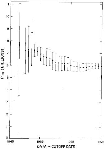
An interesting exercise8 is to determine how stable our projection
is with increasing number of data points as the years go by and what was the
earliest date at which our generalized inverse tangent function could
have precisely determined the population parameters. This is done by doing a
fit for decreasing data cutoff dates below 1975. The resulting population
parameters ![]() and
and ![]() as functions of the
data cutoff date are shown in Figure 3.
as functions of the
data cutoff date are shown in Figure 3.
 a.
a. 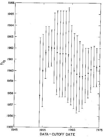 b.
b.
Fig.3.
a.
The World data single peak fit's final population
(![]() ) projection as a function of data cutoff date.
) projection as a function of data cutoff date.
b.
The World data fit's population half-data (![]() ) parameter as a function of data cutoff date.
) parameter as a function of data cutoff date.
It is seen that the
population parameters are remarkably stable with data cutoff date and
that the final population (![]() ) and half date (
) and half date (![]() ) are very well determined for data-cutoff dates as early as
1960. In other words, fits to data up to data cutoff dates beyond 1960
give good predictions for World population at future dates:
) are very well determined for data-cutoff dates as early as
1960. In other words, fits to data up to data cutoff dates beyond 1960
give good predictions for World population at future dates:
data cutoff date ![]() P(1975) prediction
P(1975) prediction
1960
6.26 ![]() 0.67 4.23
0.67 4.23
1965
6.00 ![]() 0.44
3.98
0.44
3.98
1970 5.88 ![]() 0.27
3.91
0.27
3.91
1975 5.98 ![]() 0.18
3.96
0.18
3.96
U. N. value for 1975 is 3.967
We see that the 1960 predicted value for P(1975) is 6.5% off and, from around 1965 on, the predicted value for P(1975) is less than 1.5% off. Since the generalized inverse tangent function yields such an excellent fit to the data and since its projection is excellent over the last decade, its projection into the future must be seriously considered.
A study of Figure 2 reveals that the World population parameters are precisely determined by the fit (Table 3) because the year 1975 is more than halfway up the population curve and fluctuations are not extremely large. A decline in World population growth should become visible to the naked eye in the population data graph within the next ten to fifteen years. Already there is a hint of a decline in the population growth rate (Figure 2e).
Figure 2e shows the World population growth rate for the single peak fit described above, along with the growth rate values as calculated from the population data given in Table 1. These values are rather erratic which is probably due to the poorness of the data; however, they do indicate at least two peaks in the growth rate. Our basic philosophy in fitting a single peak to the population data is that the growth rate fluctuations are short term fluctuations on a long term smooth background. However, one could adopt the philosophy that the population growth rate over a long time period is a sum of independent short term growth rate peaks; then one should fit the data with a sum of peaked functions rather than a single peaked function. If such a multi-peak fit yields peaks that are minimally overlapping, then perhaps they do represent independent phenomena. On the other band, if the peaks overlap greatly it is difficult to understand how they could be independent. So it is desirable to do a multi-peak fit to the World population data to obtain its population projection in order to compare it with the single peak fit's projection.
Such a two peak fit to the World data is given in Table 3 and shown in Figure 4.
 a.
a.  b.
b.
 c.
c.
Fig.4. The fit of a sum of two generalized-inverse tangent functions to the World population data.
a. The fit and data between 1900 and 1980.
b. The fit and growth rate values used as data in the fit from 1900 to 1980.
c. The fit and data between 1600 and 2200. The data between 1950 and 1973 are so close together that they are represented by a wide bar.
The final World population projection is 6.5 billion with an error of about one half billion, not very different than the single peak projection of 6.0 billion. The two peaks in the two peak fit do overlap considerably, so the single peak fit is probably the best projector for the future.
It is interesting to compare our two World population curves with Lester Brown's (13) timetable for achieving a stable World population of 5.8 billion by the year 2015, as is done in Table 4 and Figure 5.
Fig. 5. The two World-population fits of Table 3 along with Brown's population-stabilization timetable values (stabilization at 2015). The solid line is our single peak fit and the dashed line is our two peak fit.
Brown has described how an expansion of governmental policies and other social forces already in existence in many countries can bring about his timetable. The single peak fit to the World data reported here yields a final projection similar to Brown's, but it occurs over a longer time period; 5.8 billion occurs at about 2150. The two peak fit yields a rise similar to Brown's timetable, but projects to a higher final population (6.5 billion).
In terms of the concept of human coalition, developed by von Foerster et al.10,11,12 , that enabled the conquest of nature and thereby caused the population explosion, one can further postulate that such human coalition will enable the rapid decline in the population growth rate, shown by our fit, as the need to do so becomes more and more evident.
Our projection of a 5.98 billion final World population yields a population density of 40.2 people per square kilometer or 104 people per square mile (World land area = 148.8x10⁶ km2 = 57.47x10⁶ mi2).
For ease in comparing our projections with future World population values as they appear, in Table 5 we list the projections for our single peak fit to World population data.
Table 5. Projections of our single peak fit to World population |
|||
|
Date |
Projected Population |
Date |
Projected Population |
|
1976 |
4.01 |
1994 |
4.77 |
|
1977 |
4.07 |
1995 |
4.79 |
|
1978 |
4.12 |
1996 |
4.82 |
|
1979 |
4.18 |
1997 |
4.85 |
|
1980 |
4.23 |
1998 |
4.87 |
|
1981 |
4.28 |
1999 |
4.90 |
|
1982 |
4.32 |
2000 |
4.92 |
|
1983 |
4.37 |
2010 |
5.12 |
|
1984 |
4.41 |
2020 |
5.26 |
|
1985 |
4.45 |
2030 |
5.37 |
|
1986 |
4.49 |
2040 |
5.45 |
|
1987 |
4.53 |
2050 |
5.51 |
|
1988 |
4.57 |
2060 |
5.57 |
|
1989 |
4.61 |
2070 |
5.61 |
|
1990 |
4.64 |
2080 |
5.64 |
|
1991 |
4.67 |
2090 |
5.67 |
|
1992 |
4.71 |
2100 |
5.70 |
|
1993 |
4.74 |
|
|
Conclusion
Fitting the World population data with an asymmetric function that has a long tail (the generalized inverse tangent function) yields an excellent fit to the data and very precise values for the population parameters (final population = 6.0 billion, half date = 1960). The rise to the final population is much faster than was the rise from zero population. Our World population projection is in reasonable agreement with Brown's (13) population-stabilization timetable and Bogue's (14) 1967 prediction of an end to the population explosion. It also is in agreement with Tuerpe's (15) two sector World model.
Projection into the future of the generalized inverse tangent function fit to the World population data must be seriously considered because
1. It is an excellent fit to the data
2. It is by far the best fit that has been obtained to the data.
3. Its projection for the last decade is excellent.
Projections of national populations have been notoriously inaccurate1,2 in the past. Not enough World data were available for attempts at projections until about a decade ago. So the question that must be asked is: Will the World population projection reported here turn out to be as inaccurate as the national population projections have been? There are several reasons to think not:
· The projection over the last decade is excellent, as shown herein.
· There is no immigration or emigration component to population change.
· The sample size is much larger, i.e., idiosyncrasies of individual countries are small effects.
· Our infinite time population projection is very stable for data cutoff dates over the last fifteen years.
If the ratio of population to land area were eventually the same for the U. S. and the World, then a final World population of 6.0 billion would correspond to a final U.S. lower 48 states population of 310 million. If the U.S. to World population ratio were eventually the same as it is now a final World population of 6.0 billion would correspond to a final U.S. lower 48 states population of 320 million.
There is no cause to rejoice in our projection of a final World population of six billion, even though it is lower than other projections. Six billion is fifty percent more than the present four billion. As documented by Eckholm (16) the World's ecology is not in balance with the present population and the prognosis for the future even with no population increase is not rosy.
Acknowledgements
The author benefited from numerous discussions with Dr. Richard A. Arndt and Dr. Samuel P. Bowen. The author is grateful for the help of Mr. S. A. Goldberg, the Director of the United Nations Statistical Office, in obtaining World population values for 1974 and 1975.
14-04-99 20:12
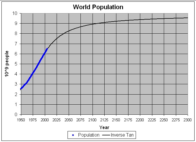
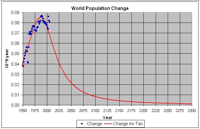
Update
The following table list the parameters for a fit of the inverse-tangent function to World population data from 1950 to 2005:
Table 3. Population parameters for fits to World population data 1950-2000 using the inverse tangent function.
![]() (*)
(*) ![]() (years) t (years)
(years) t (years)
9.91 billion people 37.01 1985.9
The following graphs show the population and population-change data for 1950-2005 and projections to 2300 for this fit.